Chapter 1: Introduction to ML System Design
1 hour 8 min readThis chapter introduces the fundamentals of designing machine learning systems at scale. It covers the key differences between traditional software systems and ML systems, and outlines the unique challenges faced when building production ML systems.
Chapter 1: Machine Learning Primer
This chapter covers the building blocks. Mastering these fundamentals is non-negotiable. An interviewer will expect you to be fluent in this language.
Topic: Feature Selection and Feature Engineering
1. One-Hot Encoding (OHE)
- Book’s Core Idea (Timeless): OHE is used for low-cardinality categorical features (e.g.,
device_type= [‘mobile’, ‘desktop’, ’tablet’]). It prevents the model from assuming a false numerical order (i.e., thattablet(2) is somehow “more” thanmobile(0)). Its major drawback is creating very wide, sparse vectors for high-cardinality features, which is memory-intensive. - The 2024+ Perspective: The principle is still valid, but its use is more limited. For any feature with more than a handful of categories (like
user_id,product_id), OHE is a non-starter. The industry has almost completely moved to embeddings for these cases. - Interview Focus & Phrasing:
- Good: “For a low-cardinality feature like ‘day_of_week’, we can use one-hot encoding.”
- Senior Level: “We’ll need to handle our categorical features. For low-cardinality ones like
country_code, one-hot encoding is a simple and effective baseline. However, for high-cardinality features likeuser_id, OHE would lead to extreme sparsity and high dimensionality. We’ll use embeddings for those instead.”
2. Mean Encoding (or Target Encoding)
- Book’s Core Idea (Timeless): Replace a category with the average value of the target variable for that category (e.g., replace ‘San Francisco’ with the average click-through rate for all users from SF). It’s a very powerful technique for tree-based models (like XGBoost) because it packs a lot of signal into a single numerical feature. The book’s warning about label leakage is its most critical point.
- The 2024+ Perspective: Still a highly relevant and powerful technique, especially in tabular data competitions (Kaggle) and for boosting models where latency isn’t the primary concern. Modern feature stores sometimes automate the robust calculation of these encodings (e.g., using out-of-fold calculations to prevent leakage).
- Interview Focus & Phrasing: Mention this as a strong option for tree-based models, but immediately bring up the risks. “We could consider target encoding for features like
city, as it can provide a strong signal to a tree-based model. However, we must be extremely careful about data leakage. To mitigate this, we’d compute the encoding on a separate dataset or use an out-of-fold strategy during training to ensure the encoding for a given row doesn’t use its own label.”
3. Feature Hashing (“The Hashing Trick”)
- Book’s Core Idea (Timeless): A technique to handle extremely high-cardinality features by hashing them into a fixed-size vector. It’s memory-efficient because you pre-define the vector size. The main drawback is hash collisions, where different features get mapped to the same index, which can hurt model performance.
- The 2024+ Perspective (Outdated): Feature hashing for model features is now largely a legacy technique. While the idea is clever, the performance loss from collisions is often not worth the memory savings, especially when compared to embeddings. Modern hardware and frameworks can handle large embedding tables more gracefully.
- Interview Focus & Phrasing: Acknowledge it historically. “In the past, for systems with millions of features like in AdTech, feature hashing was a common way to manage memory. It’s a trade-off between memory and performance due to collisions. Today, we’d almost always prefer to learn a dedicated embedding layer, as it captures semantic relationships and avoids collisions, leading to better model performance.”
4. Cross Features
- Book’s Core Idea (Timeless): Explicitly combining two or more categorical features to capture their interaction (e.g.,
feature_A=‘USA’ +feature_B=‘iPhone’ ->crossed_feature=‘USA_iPhone’). This helps linear models and shallow networks learn relationships they otherwise couldn’t. The book’s reference to Wide & Deep is the classic example. - The 2024+ Perspective: The concept of capturing feature interactions is more important than ever. The method has evolved. While Wide & Deep is still a valid pattern, modern architectures like Transformers (with their self-attention mechanism) are exceptionally good at learning these interactions implicitly from the raw feature embeddings. You don’t always need to manually define the crosses.
- Interview Focus & Phrasing: Focus on the “why.” “A key challenge in this problem is capturing the interaction between features, for example, a user’s country and their device type. A classic approach is the Wide & Deep model, where we’d manually create cross-product transformations for the ‘wide’ part. A more modern approach would be to feed the embeddings for all features into a deep network, perhaps with a cross-network layer like DCN or an attention mechanism, which can learn these interactions automatically.”
5. Embedding
- Book’s Core Idea (Timeless): This is the most important feature engineering technique in the book and in modern ML. An embedding is a dense, low-dimensional, learned vector representation of a categorical feature. The book correctly explains the two main ways to get them:
- Co-trained: Learning the embedding as part of your main model (e.g., an embedding layer in Keras/PyTorch).
- Pre-trained: Learning the embedding separately on a different task (e.g., Word2Vec on text, or node2vec on a graph) and then using it as a static feature.
- The 2024+ Perspective: This is the heart of modern ML.
- The Rise of Foundation Models: The “pre-trained” paradigm now dominates. You don’t just use Word2Vec; you use embeddings from massive, powerful foundation models (e.g., OpenAI’s
text-embedding-3-large, Sentence-BERT, or image embeddings from CLIP). Your job is less about designing the pre-training task and more about choosing the right foundation model. - The Two-Tower Model: The book’s description of the two-tower model for retrieval (e.g., at YouTube) is still State-of-the-Art for recommendation and search. This is a critical pattern to know inside and out.
- The Rise of Foundation Models: The “pre-trained” paradigm now dominates. You don’t just use Word2Vec; you use embeddings from massive, powerful foundation models (e.g., OpenAI’s
- Interview Focus & Phrasing: This should be your default answer for high-cardinality features.
- “For user IDs and item IDs, we will learn dense embedding vectors. This allows the model to capture semantic similarities—for instance, users who buy similar products will have similar vectors.”
- For a retrieval system, you must bring up the two-tower model. “We’ll design a two-tower retrieval model. The query tower will ingest user features and produce a query embedding. The candidate tower will ingest item features and produce an item embedding. At training time, we’ll optimize these towers using a contrastive loss so that the dot product between a user and a relevant item is high. For serving, we can pre-compute all item embeddings and put them into a vector index for efficient retrieval.”
Here is the diagram for the Two-Tower Model, which is central to this discussion.
graph TD
    subgraph "Query Tower"
        U_Features[User Features<br/>context, history] --> U_L1(Dense Layer)
        U_L1 --> U_L2(Dense Layer)
        U_L2 --> QueryEmbedding[Query Embedding]
    end

    subgraph "Candidate Tower"
        I_Features[Item Features<br/>metadata, text] --> I_L1(Dense Layer)
        I_L1 --> I_L2(Dense Layer)
        I_L2 --> ItemEmbedding[Item Embedding]
    end

    subgraph "Training Objective"
        QueryEmbedding -- Dot Product --> Score
        ItemEmbedding -- Similarity --> Score
        Score --> Loss(Contrastive Loss<br/>e.g., Softmax, Hinge)
    end

    subgraph "Serving / Inference"
        direction LR
        ItemEmbedding --> AllItemEmbeddings[Pre-computed<br/>Item Embeddings]
        AllItemEmbeddings --> ANN_Index[(Vector Database / FAISS<br/>Approximate Nearest Neighbor)]
        QueryEmbedding --> ANN_Index
        ANN_Index --> Top_K_Candidates[Top K Candidates]
    end

    style QueryEmbedding fill:#cde4ff
    style ItemEmbedding fill:#dff0d8
Excellent. Let’s dive into the next section of Chapter 1. We’ll cover Training Pipelines, Handling Imbalance, and Data Generation/Splitting. These topics are less about the model itself and more about the crucial data infrastructure that makes modeling possible at scale.
Topic: Training Pipeline & Data Partitioning (Page 33)
Book’s Core Idea (Timeless): To train models on massive datasets (terabytes or petabytes), you can’t just load a CSV file. The book correctly identifies two key strategies:
- Columnar Storage (Parquet, ORC): Instead of storing data row-by-row like in a CSV, columnar formats store it column-by-column. Why this matters: ML training jobs often only need a subset of columns. Columnar formats let you read only the columns you need, dramatically reducing I/O and speeding up data loading. This is a fundamental concept in big data.
- Data Partitioning: Breaking up the data into a logical directory structure, almost always by date (e.g.,
/year=2024/month=05/day=21/). Why this matters: It allows the query engine to completely skip reading data from partitions that aren’t relevant to your query (e.g., “give me the last 7 days of data”). This is called “predicate pushdown” and it’s a massive performance win.
The 2024+ Perspective (Modern Augmentation): The principles are solid, but the ecosystem built on top has become standard.
- The Rise of Table Formats (Iceberg/Delta Lake): The biggest change is the widespread adoption of open table formats like Apache Iceberg and Delta Lake. These are layers that sit on top of your Parquet files in the data lake. They solve critical problems that raw Parquet files don’t:
- ACID Transactions: They prevent you from reading corrupted or incomplete data if a write job fails midway. This is huge for data reliability.
- Schema Evolution: They make it safe to add/remove/rename columns without breaking downstream jobs.
- Time Travel: They allow you to query the state of your data at a specific point in time, which is invaluable for debugging and reproducing experiments.
- Orchestration: Training pipelines aren’t run manually. They are scheduled and managed by orchestrators. Airflow is the industry veteran, but newer tools like Dagster and Prefect are gaining traction by offering better data awareness and local development experiences.
- The Rise of Table Formats (Iceberg/Delta Lake): The biggest change is the widespread adoption of open table formats like Apache Iceberg and Delta Lake. These are layers that sit on top of your Parquet files in the data lake. They solve critical problems that raw Parquet files don’t:
Interview Focus & Phrasing:
- Good: “We will store our training data in a data lake like S3, using the Parquet format and partitioning by date.”
- Senior Level: “We’ll design a daily batch training pipeline orchestrated by Airflow. The pipeline’s source data will reside in our data lake (S3) and be managed by an open table format like Apache Iceberg. This gives us transactional guarantees and schema safety. The training job itself, running on a Spark cluster, will read the last 90 days of data, leveraging Iceberg’s partition pruning for efficiency, compute the necessary features, and then train the model.”
Here’s a diagram illustrating this modern training pipeline:
graph TD
    subgraph datasources["Data Sources"]
        Logs[Log Files]
        DB[(Production DB)]
    end

    subgraph pipeline["Daily Batch Pipeline"]
        direction LR
        Ingest[Ingestion Job Spark] --> Lake[Data Lake with<br/>Apache Iceberg Tables]
        Lake -- "Reads last N days" --> FeatEng[Feature Engineering Job Spark]
        FeatEng --> TrainJob[Model Training Job<br/>PyTorch/XGBoost on Spark]
        TrainJob --> ModelRegistry[(Model Registry<br/>MLflow, SageMaker)]
    end

    Logs --> Ingest
    DB --> Ingest

    style Lake fill:#cde4ff,stroke:#333,stroke-width:2px
Mapping Generic Concepts to AWS Services
Let’s break down the AWS equivalent of that senior-level answer and build a concrete diagram around a common use case: Training a daily model for a Recommendation System.
| Generic Concept | AWS Primary Service(s) | Role / “Why” you use it |
|---|---|---|
| Data Lake Storage | Amazon S3 (Simple Storage Service) | The foundation. It’s the cheap, durable, and scalable object store where you dump all your raw and processed data (like Parquet files). |
| Table Format | AWS Glue Data Catalog (as the metastore) + Apache Iceberg/Hudi | Glue Data Catalog acts as the central “address book” for your data lake. It stores the metadata (schema, location, partitions) for your tables. Iceberg (or Hudi) manages the actual data files within S3, providing the ACID transactions, time travel, and schema evolution we discussed. |
| Data Querying / Ad-hoc Analysis | Amazon Athena | A serverless query engine that lets you run standard SQL directly on your data in S3 using the Glue Data Catalog. This is how data scientists explore the data without spinning up a cluster. |
| ETL / Feature Engineering | AWS Glue (for serverless Spark jobs) or Amazon EMR (for managed Spark/Hadoop clusters) | Glue is great for simpler, serverless ETL jobs. EMR is for heavy-duty, long-running Spark jobs where you need more control over the cluster configuration. Both are used for the heavy lifting of data transformation. |
| Pipeline Orchestration | Amazon MWAA (Managed Workflows for Apache Airflow) | This is the AWS-managed version of Airflow. It’s the “conductor” that defines the dependencies between your jobs (e.g., “Run the feature engineering job only after the daily data ingestion job succeeds”) and schedules them. |
| Model Training | Amazon SageMaker Training | The service for running training jobs at scale. It handles spinning up the necessary compute instances (with GPUs if needed), running your training script (e.g., PyTorch, TensorFlow), and saving the final model artifact back to S3. |
| Model Registry | Amazon SageMaker Model Registry | A centralized repository to version, approve, and manage your trained models before they are deployed. It’s crucial for governance and reproducibility. |
What about Snowflake? Snowflake is a cloud data warehouse, not a data lake tool in this context. While it can connect to S3, it represents a different architectural pattern. The “modern data stack” we’re describing here is centered on an open data lakehouse architecture (S3 + Iceberg + Spark), which is more common for large-scale ML training pipelines because it’s more flexible and cost-effective for unstructured and semi-structured data. Mentioning Snowflake is fine, but the S3/Glue/Spark stack is the more direct AWS equivalent.
Use Case Diagram: Daily Re-training of a “Products You May Like” Model on AWS
Here is the diagram showing how these services fit together in a production pipeline.
graph TD
    subgraph "Data Sources"
        A[App & Web Logs<br/>via Kinesis Firehose]
        B[S3 Raw Data Bucket]
        C[Production DB<br/>e.g., RDS, DynamoDB]
        D[Daily DB Snapshots]
    end

    subgraph "Orchestration Layer: Amazon MWAA Airflow"
        P1(DAG Starts<br/>Daily @ 1 AM)
    end

    subgraph "ETL & Feature Engineering Layer"
        S3_Lakehouse[S3 Data Lakehouse<br/>Storage: Parquet Files<br/>Format: Apache Iceberg<br/>Metastore: AWS Glue Data Catalog]
        Glue_Job[AWS Glue ETL Job<br/>Spark]
    end

    subgraph "Model Training & Registration Layer"
        SageMaker_Train[SageMaker Training Job<br/>PyTorch]
        SageMaker_Registry[(SageMaker Model Registry)]
    end

    subgraph "Analytics & Exploration"
        Athena[Amazon Athena]
    end

    A --> B
    C --> D
    D --> B
    B --> Glue_Job
    Glue_Job --> S3_Lakehouse
    S3_Lakehouse --> SageMaker_Train
    SageMaker_Train --> SageMaker_Registry
    Athena --> S3_Lakehouse
    P1 --> Glue_Job
    P1 --> SageMaker_Train
    P1 --> SageMaker_Registry

    style S3_Lakehouse fill:#cde4ff,stroke:#333,stroke-width:2px
    style Glue_Job fill:#fff0b3,stroke:#333,stroke-width:2px
    style SageMaker_Train fill:#dff0d8,stroke:#333,stroke-width:2px
    style Athena fill:#f5c6cb,stroke:#333,stroke-width:2px
Explaining the Diagram in an Interview
“Here’s how I would architect the daily training pipeline on AWS for our recommendation model.
Orchestration: The entire process would be managed by a DAG in Amazon MWAA (Airflow), scheduled to run daily.
Ingestion: Raw data, like clickstream logs from Kinesis and daily snapshots from our production RDS database, lands in a dedicated S3 bucket.
ETL & Feature Store Creation: Our first Airflow task kicks off an AWS Glue ETL job. This serverless Spark job reads the raw data, cleans and transforms it, computes our features, and writes the output as partitioned Parquet files back to our main S3 data lake. We’ll use the AWS Glue Data Catalog as a metastore with the Apache Iceberg format. This gives us ACID compliance, so downstream jobs never read partial data, and allows our data science team to query the data easily with Athena.
Model Training: Once the Glue job succeeds, Airflow triggers the next task: a SageMaker Training Job. SageMaker pulls our training script, provisions the necessary compute (e.g., GPU instances), reads the clean feature data directly from our S3 data lakehouse, and trains the model.
Model Registration: After training, the final model artifact is versioned and saved to the SageMaker Model Registry. This creates a golden copy, tracks its performance metrics, and puts it in a ‘pending approval’ state before it can be deployed to production. This CI/CD for ML approach is crucial for safe and reproducible deployments.”
Topic: Handle Imbalance Class Distribution (Page 34)
Book’s Core Idea (Timeless): This is a classic problem in domains with rare events (ad clicks, fraud). The book gives the three canonical solutions:
- Class Weighting: The simplest and often best first step. Penalize errors on the minority class more heavily in your loss function.
- Downsampling (Majority Class): When you have massive data (e.g., billions of non-clicks), you can throw away a large, random portion to make the training problem more manageable. This is the standard in big tech.
- Oversampling (Minority Class) / SMOTE: For smaller datasets where every positive example is precious. SMOTE creates synthetic minority class examples. Less common in large-scale systems. The book’s most important warning is to NEVER resample your validation/test set. They must reflect reality.
The 2024+ Perspective (Modern Augmentation):
- The Calibration Imperative: This is the critical piece that senior candidates must discuss. When you downsample, you change the baseline probability in your training data (e.g., from 1% clicks to 50% clicks). The model’s raw output
pwill be biased high. You need to correct for this before the prediction can be used for anything quantitative (like bidding in an ad auction). The formula is essential:calibrated_p = p / (p + (1-p) / w)wherewis the downsampling rate (e.g., if you kept 10% of negatives, w=0.1). - Focal Loss: As mentioned before, Focal Loss is a more advanced alternative to simple class weighting. It’s an excellent talking point to show you know modern techniques.
- The Calibration Imperative: This is the critical piece that senior candidates must discuss. When you downsample, you change the baseline probability in your training data (e.g., from 1% clicks to 50% clicks). The model’s raw output
Interview Focus & Phrasing:
- Good: “This is an imbalanced problem, so I’ll downsample the negative class in the training set.”
- Senior Level: “This is a classic class imbalance problem. We have several strategies. I’d start with class weighting, as it’s non-invasive. If performance is still an issue, we can move to downsampling the negative class. This is computationally efficient, but it requires a crucial post-processing step: we must calibrate the model’s outputs to correct for the artificial sampling rate before they are used downstream. Our validation set will, of course, maintain the original, un-sampled distribution to give us a true measure of performance.”
Topic: Data Generation Strategy & How to Split Train/Test Data (Pages 36, 39)
Book’s Core Idea (Timeless):
- Getting Labels: How do you get initial labels? The book gives great examples: use chronological feeds, use existing user actions (“likes” are positive, items they saw but skipped are negative), or use proxy signals (LinkedIn using
skillsto recommendcourses). - Splitting Data: The most important rule is that for any time-series problem (forecasting, user behavior models), you must not split randomly. A random split would cause data leakage by using future information to train a model that predicts the past. You must use a time-based split (e.g., train on January, validate on February). The book’s examples of Sliding Window and Expanding Window for backtesting are perfect.
- Getting Labels: How do you get initial labels? The book gives great examples: use chronological feeds, use existing user actions (“likes” are positive, items they saw but skipped are negative), or use proxy signals (LinkedIn using
The 2024+ Perspective (Modern Augmentation):
- Negative Sampling is a Design Choice: The book treats “negative labels” as something you just find. In modern recommender systems, particularly with two-tower models, the choice of which negatives to use during training is a key modeling decision.
- Easy Negatives: Randomly sampled items.
- Hard Negatives: Items that are “close” to the positive item in the embedding space but the user didn’t click. Training on these helps the model learn finer distinctions. YouTube’s papers talk extensively about the importance of hard negative mining.
- User-based Splitting: For personalization problems, another important splitting strategy is to split by user. You hold out a set of users entirely to test how the model performs on users it has never seen before (the “cold start” problem).
- Negative Sampling is a Design Choice: The book treats “negative labels” as something you just find. In modern recommender systems, particularly with two-tower models, the choice of which negatives to use during training is a key modeling decision.
Interview Focus & Phrasing:
- Good: “We’ll split our data by time. We’ll train on one month and test on the next day.”
- Senior Level: “Our splitting strategy is critical to avoid leakage. We will use a strict temporal split, for example, training on data up to day T and validating on day T+1. For our two-tower retrieval model, we need to be thoughtful about negative sampling. We’ll start with random in-batch negatives, but to improve performance, we would implement a strategy for hard negative mining to help the model learn the subtle differences between similar items. To evaluate cold-start performance, we’ll also maintain a holdout set of users.”
Of course. Let’s slow down and unpack these concepts properly. This is the core of what separates a junior from a senior MLE. We will go deep into each one, with the goal of you being able to explain it with the same level of clarity and intuition.
Topic : Loss Functions - The “Why” Behind Optimization
A loss function is the mathematical objective your model minimizes during training. It’s the most direct way you, the engineer, tell the model what “good” looks like.
Deep Dive 1: Regression Loss: How wrong is our number?
A. MSE vs. MAE: The Outlier Dilemma
Let’s imagine we’re predicting house prices.
- Target Price: $300k
- Model A Prediction: $310k (Error: $10k)
- Model B Prediction: $350k (Error: $50k)
Now, let’s see how MSE and MAE treat these errors.
Mean Absolute Error (MAE): The penalty is linear with the error.
- Equation:
MAE = (1/n) * Σ |y_true - y_pred| - Intuition: It answers “On average, how far off are our predictions in dollars?”
- Calculation:
- Model A’s MAE contribution:
|$300k - $310k| = $10k - Model B’s MAE contribution:
|$300k - $350k| = $50k
- Model A’s MAE contribution:
- Conclusion: The error from Model B ($50k) is exactly 5 times worse than the error from Model A ($10k). This feels intuitive.
Mean Squared Error (MSE): The penalty grows quadratically with the error.
- Equation:
MSE = (1/n) * Σ (y_true - y_pred)² - Intuition: It answers “What’s the average of the squared errors?” It doesn’t have an intuitive unit, which is why we often use RMSE (Root Mean Squared Error =
√MSE) to bring it back to the original units (dollars). - Calculation:
- Model A’s MSE contribution:
($10k)² = 100,000,000 - Model B’s MSE contribution:
($50k)² = 2,500,000,000
- Model A’s MSE contribution:
- Conclusion: The error from Model B is 25 times worse than the error from Model A. MSE despises large errors and will aggressively tune the model to avoid them, even at the cost of being slightly worse on other, smaller errors.
graph TD
    subgraph "MAE (Linear Penalty)"
        A[Error of $10k] --> B(Penalty = 10k)
        C[Error of $50k] --> D(Penalty = 50k)
    end

    subgraph "MSE (Quadratic Penalty)"
        E[Error of $10k] --> F(Penalty = 100M)
        G[Error of $50k] --> H(Penalty = 2,500M)
    end

    style D fill:#f5c6cb
    style H fill:#f5c6cb
Senior Takeaway: Choose MSE when outliers are “real” errors you must avoid (e.g., predicting stress on a bridge beam). Choose MAE when outliers might be measurement noise and you don’t want them to dominate the model’s training.
B. Quantile Loss: When Over vs. Under Matters
Imagine we’re DoorDash, estimating food delivery time.
- Case 1 (Over-prediction): We predict 30 mins, food arrives in 25 mins. Result: Happy, pleasantly surprised customer.
- Case 2 (Under-prediction): We predict 30 mins, food arrives in 35 mins. Result: Unhappy, frustrated customer who might not order again.
Clearly, under-prediction is more costly. We want our model to “know” this. This is where Quantile Loss comes in.
- Equation:
Quantile Loss = Σ q * |y_true - y_pred|(if error is positive, i.e., under-prediction)+ Σ (1-q) * |y_true - y_pred|(if error is negative, i.e., over-prediction). Hereqis the quantile. - Intuition: It’s just a weighted MAE. You choose the weights.
- Example (q = 0.8):
- We want 80% of our predictions to be over-estimates or correct.
- If we predict 30 mins and it arrives in 35 (under-prediction), the error of 5 mins is multiplied by
q = 0.8. Loss =5 * 0.8 = 4.0. - If we predict 30 mins and it arrives in 25 (over-prediction), the error of -5 mins is multiplied by
(1-q) = 0.2. Loss =5 * 0.2 = 1.0.
- The model now learns it’s 4 times more painful to be late than to be early. It will naturally start “padding” its estimates to avoid the larger penalty.
Deep Dive 2: Classification Loss: How wrong is our label?
A. Contrastive Loss: Learning by Comparison
This is the key to all modern retrieval systems (search, recommendation, RAG). Forget predicting a single score for a moment. The goal is to produce an embedding (a vector) for the user and for every item, such that the vectors of “good” pairs are close together.
The Setup: Imagine a mini-batch of training data for a YouTube recommender. It contains one “positive” pair:
(User A, Video_SciFi_1)because User A watched it. It also contains several “negative” pairs, which are just the other videos in the batch:(User A, Video_Cooking_2),(User A, Video_Sports_3).The Goal: We want to make the similarity score (often dot product) of the positive pair much higher than the similarity scores of the negative pairs.
Sim(User_A_vec, Video_SciFi_1_vec)should be »Sim(User_A_vec, Video_Cooking_2_vec)Sim(User_A_vec, Video_SciFi_1_vec)should be »Sim(User_A_vec, Video_Sports_3_vec)
How it Works (In-batch Softmax, a common contrastive loss):
- Calculate the similarity score
s_ifor every user-item pair in the batch. - Treat it like a classification problem! Apply a Softmax function across all the scores.
- The loss is simply the Cross-Entropy loss of trying to “classify” the positive pair as the correct one.
- Calculate the similarity score
Equation (Conceptual):
Loss = -log( exp(s_positive) / (exp(s_positive) + Σ exp(s_negative)) )Why it’s genius: By minimizing this loss, you are implicitly pushing the positive score up and all the negative scores down, achieving the goal of separating them in the embedding space. This is how the two-tower model is trained.
graph LR
    subgraph "Embedding Space"
        direction BT
        U(User)
        P((Positive<br/>Item))
        N1((Negative<br/>Item))
        N2((Negative<br/>Item))

        U -- "Pull Closer" --> P
        U -- "Push Away" --> N1
        U -- "Push Away" --> N2
    end

    CL(Contrastive Loss)
    CL --> U
    CL --> P
    CL --> N1
    CL --> N2

    style P fill:#dff0d8
    style N1 fill:#f5c6cb
    style N2 fill:#f5c6cb
Senior Takeaway: When designing a system with a retrieval step, you must talk about using a contrastive loss to train the embedding models (the two towers).
Deep Dive 3: Huber Loss: The Robust “Best of Both Worlds”
Book’s Core Idea (Timeless): Huber Loss is designed as a composite function to get the best attributes of both MSE and MAE. For small errors, it uses a quadratic function (like MSE), which is strongly convex and leads to stable convergence. For large errors, it switches to a linear function (like MAE), which prevents outliers from dominating the gradient and pulling the model too far off course.
Intuition & Equation: It’s defined by a threshold hyperparameter,
δ(delta). You, the engineer, decide what constitutes a “small” vs. “large” error.The loss is defined piecewise:
- If
|y_true - y_pred| <= δ:Loss = 1/2 * (y_true - y_pred)²(It’s MSE) - If
|y_true - y_pred| > δ:Loss = δ * |y_true - y_pred| - 1/2 * δ²(It’s MAE, with a constant adjustment to make the function smooth at theδboundary)
- If
Example: Let’s set
δ = 1.0. We’re predicting a value of 10.- Prediction 1 = 10.5 (Error = 0.5): Since
0.5 <= δ, we use the MSE part. Loss =0.5 * (0.5)² = 0.125. - Prediction 2 = 13.0 (Error = 3.0): Since
3.0 > δ, we use the MAE part. Loss =1.0 * 3.0 - 0.5 * (1.0)² = 2.5. - Notice that a pure MSE would have given a loss of
(3.0)² = 9.0. Huber loss provides a much smaller, more reasonable penalty.
- Prediction 1 = 10.5 (Error = 0.5): Since
The 2024+ Perspective: Huber Loss remains a fantastic, practical choice for many regression problems. Its main drawback is simply the need to tune the
δhyperparameter. In libraries like XGBoost and LightGBM, it’s often available as a built-in objective function. It signals that you are thinking about the robustness of your training process.Interview Phrasing: “For this regression task, I’d start with Huber loss instead of a simple MSE. This would make our training process more robust to potential outliers in the data, which are common in real-world datasets. We would need to tune the delta hyperparameter, likely via cross-validation, to define the point at which we treat an error as an outlier.”
graph TD
    subgraph "Error Size"
        A[Small Error<br/>error <= δ]
        B[Large Error<br/>error > δ]
    end

    subgraph "Huber Loss Behavior"
        C[Quadratic Penalty<br/>Like MSE]
        D[Linear Penalty<br/>Like MAE]
    end

    A --> C
    B --> D

    C --> E[Result: Stable convergence<br/>for common cases]
    D --> F[Result: Robust to outliers]

    style C fill:#dff0d8
    style D fill:#f5c6cb
Deep Dive 4: How Facebook Uses Normalized Cross Entropy (NCE): The “Fair Comparison” Metric
Book’s Core Idea (Timeless): The book presents a crucial real-world problem: how do you compare the performance of two models that operate in different environments? Normal Log Loss is not a fair comparison.
- Problem: Imagine you have Model A for US ads (base CTR = 2%) and Model B for Indian ads (base CTR = 0.5%). Model A achieves a log loss of 0.10. Model B achieves a log loss of 0.04. Is Model B better? Not necessarily! It’s much easier to get a low log loss on a dataset with very low base probability.
Intuition & Equation: NCE re-frames the question from “What is the model’s log loss?” to “How much better is the model than a dumb baseline that always predicts the average?”
NCE = LogLoss(model) / LogLoss(background_rate)Where
LogLoss(background_rate)is the cross-entropy you’d get if your model just predicted the average CTR for every single example.- Interpretation:
NCE < 1.0: Your model is smarter than the baseline. The lower, the better.NCE = 1.0: Your model is exactly as good as the baseline.NCE > 1.0: Your model is actively worse than just predicting the average.
- Interpretation:
Example (from the book):
- Model 1 (Fixed Prediction) has a log loss of 0.36 on data with 10% CTR. The baseline log loss is 0.325.
NCE = 0.36 / 0.325 = 1.11. This model is worse than just guessing the average. - Model 2 (Fancy Model) has a log loss of 0.65 on data with 50% CTR. The baseline log loss is 0.693.
NCE = 0.65 / 0.693 = 0.945. This model is better than guessing the average. - Conclusion: The fancy model is the “smarter” model, even though its absolute log loss was higher.
- Model 1 (Fixed Prediction) has a log loss of 0.36 on data with 10% CTR. The baseline log loss is 0.325.
The 2024+ Perspective: This concept is a hallmark of a mature ML practice. It’s used for comparing models across different countries, platforms (iOS vs. Android), or any segment with a different underlying target distribution. It’s a fantastic point to bring up in a discussion about offline evaluation.
Interview Phrasing: “When evaluating our click prediction model across different regions, simply comparing log loss can be misleading due to varying background CTRs. I would implement Normalized Cross-Entropy (NCE) as a key offline metric. This would allow us to measure the ’lift over baseline’ for each model in its respective domain, giving us a fair and comparable measure of model intelligence.”
Deep Dive 4: Forecast Metrics: MAPE and SMAPE
- Book’s Core Idea (Timeless): These metrics are used when you care about relative error (percentage) rather than absolute error. This is useful for comparing forecast accuracy on items with different scales (e.g., forecasting sales of a $1000 TV vs. a $10 pack of batteries).
- Mean Absolute Percentage Error (MAPE):
- Equation:
MAPE = (100%/n) * Σ |(Actual - Forecast) / Actual| - The Big Flaw (Asymmetry): MAPE has a different range for over-forecasting vs. under-forecasting.
- If
Actual = 100,Forecast = 50->|50/100|= 50% error. - If
Actual = 100,Forecast = 150->|-50/100|= 50% error. - If
Actual = 100,Forecast = 0(max under-forecast) ->|100/100|= 100% error. - If
Actual = 100,Forecast = 300->|-200/100|= 200% error.
- If
- The penalty for over-forecasting is unbounded, while the penalty for under-forecasting is capped at 100%. This means a model trained to minimize MAPE will learn to be biased towards under-forecasting. It also blows up if
Actualis zero.
- Equation:
- Symmetric Absolute Percentage Error (SMAPE):
- Equation:
SMAPE = (100%/n) * Σ |Forecast - Actual| / ((|Actual| + |Forecast|)/2) - The Fix: It attempts to fix the asymmetry by normalizing by the average of the actual and forecast values. This bounds the metric between 0% and 200%.
- The New Problem: The interpretation is less intuitive, and it can still be unstable if both Actual and Forecast are very close to zero.
- Equation:
- The 2024+ Perspective: While commonly found in business reports due to their intuitive nature, these metrics are often avoided as direct loss functions for training because of their instability. A more common approach in serious forecasting systems is to:
- Transform the data: Take the
log(1 + target). - Train the model: Use a stable loss like MAE or Huber on the transformed data.
- Inverse transform: Exponentiate the model’s predictions to get back to the original scale.
- Report: Calculate MAPE/SMAPE on the final predictions for business stakeholders.
- Transform the data: Take the
- Interview Phrasing: “For reporting forecast accuracy to our business partners, MAPE is a good choice because percentage error is easy to understand. However, for the model’s objective function, I would avoid MAPE due to its known asymmetry and instability. A more robust approach is to train on the log-transformed sales data using a simple MAE loss, and then report MAPE on the final, inverse-transformed predictions.”
Deep Dive 5: Focal Loss: Focusing on the Hard Cases
Book’s Core Idea (Timeless): Focal Loss is an improvement on standard Cross-Entropy for cases with extreme class imbalance, especially when there are many “easy” examples that dominate the loss. Its canonical use case is object detection, where the vast majority of pixels in an image are “easy background.”
Intuition & Equation: It adds a modulating factor
(1 - p_t)^γto the cross-entropy loss.Focal Loss = - (1 - p_t)^γ * log(p_t)p_t: The model’s predicted probability for the ground-truth class.γ(gamma): The focusing parameter (e.g.,γ = 2).
Example:
- Easy Example: The model is very confident about a correct prediction,
p_t = 0.99. The modulating factor is(1 - 0.99)² = 0.0001. The loss for this example is almost zeroed out. - Hard Example: The model is very unsure,
p_t = 0.1. The modulating factor is(1 - 0.1)² = 0.81. The loss for this example is only slightly reduced.
- Easy Example: The model is very confident about a correct prediction,
The Result: The model is freed from wasting its capacity on perfecting its confidence for easy examples and can focus its updates on learning the hard ones.
graph TD
    subgraph "Standard Cross-Entropy"
        Easy[Easy Example<br/>p=0.99] --> Loss_Easy_CE[Loss = 0.01]
        Hard[Hard Example<br/>p=0.1] --> Loss_Hard_CE[Loss = 2.3]
        Loss_Hard_CE -- "230x larger" --> Loss_Easy_CE
    end

    subgraph "Focal Loss (γ=2)"
        Easy2[Easy Example<br/>p=0.99] --> Loss_Easy_FL[Loss ≈ 0.0001]
        Hard2[Hard Example<br/>p=0.1] --> Loss_Hard_FL[Loss ≈ 1.86]
        Loss_Hard_FL -- "~18,600x larger" --> Loss_Easy_FL
    end

    Title1[Total loss is dominated by<br/>a huge number of easy examples]
    Title2[Total loss is dominated by<br/>the few, hard examples]
- The 2024+ Perspective: Focal loss remains a very important and widely recognized technique. Mentioning it shows you are familiar with advanced solutions to the common class imbalance problem.
- Interview Phrasing: “Given the extreme imbalance between clicked and non-clicked ads, a simple weighted cross-entropy might not be enough. The loss could be dominated by the millions of easily-classified non-clicks. I would experiment with Focal Loss. By setting a gamma value, we can dynamically down-weight the loss for these easy examples and force the model to focus its capacity on the much smaller and harder-to-predict set of positive clicks.”
Deep Dive 6: Hinge Loss: Learning with a Margin
Book’s Core Idea (Timeless): Hinge loss is primarily associated with Support Vector Machines (SVMs). Its goal is not just to get the classification right, but to get it right with a high degree of confidence. It introduces the concept of a “margin.”
Intuition & Equation: It operates on raw scores (not probabilities) and uses labels of
{-1, +1}.Loss = max(0, 1 - y_true * y_pred)Example: The margin is at
+1for positive classes and-1for negative classes.- Case 1 (Correct, Confident):
y_true = 1,y_pred = 1.5. Loss =max(0, 1 - 1*1.5) = 0. No penalty. The point is outside the margin. - Case 2 (Correct, Not Confident):
y_true = 1,y_pred = 0.6. Loss =max(0, 1 - 1*0.6) = 0.4. It’s penalized because it’s correct but falls inside the margin. - Case 3 (Incorrect):
y_true = 1,y_pred = -0.5. Loss =max(0, 1 - 1*(-0.5)) = 1.5. Heavily penalized.
- Case 1 (Correct, Confident):
The 2024+ Perspective: While classic SVMs are less used, Hinge Loss is very relevant today as a form of contrastive loss. It’s excellent for training retrieval models. You can formulate a Triplet Loss using it:
Loss = max(0, margin - Sim(anchor, positive) + Sim(anchor, negative)). This loss function directly optimizes to ensure the similarity of a positive pair is greater than the similarity of a negative pair by at leastmargin.Interview Phrasing: “While Hinge Loss is classically from SVMs, its ‘margin’ concept is very useful in modern systems. For our two-tower retrieval model, we could use a hinge-based triplet loss. This would train the model to ensure that the dot product of a user with a relevant item is greater than the dot product with an irrelevant item by a specific, pre-defined margin, leading to a more robust separation in the embedding space.”
Topic: Model Evaluation Metrics
Area Under the Curve (AUC): The “Better than Chance?” Metric
- Book’s Core Idea (Timeless): AUC, specifically for the Receiver Operating Characteristic (ROC) curve, is one of the most fundamental metrics for binary classification. It answers a single, powerful question: “If I randomly pick one positive example and one negative example, what is the probability that my model assigned a higher score to the positive one?”
- Intuition & How it’s built:
- Your model doesn’t output 0s and 1s. It outputs a continuous score (e.g., 0.0 to 1.0).
- To make a decision, you need a threshold. (e.g., “If score > 0.5, classify as 1”).
- The ROC curve is generated by plotting the True Positive Rate (TPR) against the False Positive Rate (FPR) for every possible threshold.
- TPR (Recall):
True Positives / (True Positives + False Negatives)-> “Of all the actual positives, how many did we find?” - FPR:
False Positives / (False Positives + True Negatives)-> “Of all the actual negatives, how many did we incorrectly label as positive?”
- TPR (Recall):
- AUC is the literal area under this curve.
graph TD
    subgraph "ROC Curve"
        direction LR
        A((0,0)) -- "Threshold=1.0<br/>Catch nothing" --> B(Model's Curve)
        B -- "Threshold=0.0<br/>Catch everything" --> C((1,1))
        A -- "Random Guessing<br/>AUC = 0.5" --> C
        D((0,1))
        style D fill:#dff0d8,stroke-width:4px,stroke:green
        X_AXIS --- Y_AXIS
    end

    subgraph Legend
        Ideal["Perfect Model<br/>Point (0,1)"]
        Good["Good Model<br/>Curve bows to top-left"]
        Random["Random Model<br/>Diagonal Line"]
    end

    Y_AXIS[True Positive Rate]
    X_AXIS[False Positive Rate]
- Interpretation:
AUC = 1.0: Perfect classifier.AUC = 0.5: Useless classifier, equivalent to a random guess.AUC = 0.0: Perfectly wrong classifier (it’s always predicting the opposite).
- The 2024+ Perspective: AUC’s main strength is that it’s threshold-independent. It evaluates the quality of your model’s scoring without you having to first pick a decision threshold. However, its weakness is that it can be misleading on highly imbalanced datasets. For a dataset with 99.9% negatives, a model can get a very high AUC by just being good at identifying negatives. This is why Precision-Recall AUC (PR-AUC) is often preferred in these imbalanced cases.
- Interview Phrasing: “To get a high-level view of my classifier’s discriminative power, I would start by measuring the ROC AUC. This gives us a threshold-independent measure of separability. However, since this is a highly imbalanced ad-click problem, I would also closely monitor the Precision-Recall AUC, as it provides a better picture of performance on the rare positive class, which is our primary business interest.”
Mean Average Recall at K (MAR@K): The “Did we find everything?” Metric
- Book’s Core Idea (Timeless): As we discussed, this is for the retrieval/candidate generation stage. But what if you have a list of users? MAR@K is simply the average of the Recall@K values across all your users.
- Equation:
MAR@K = (1/|U|) * Σ (for each user u in U) Recall@K(u)- Where
|U|is the total number of users.
- Where
- Example:
- User 1: We found 7 of their 10 relevant items.
Recall@K = 0.7. - User 2: We found 4 of their 5 relevant items.
Recall@K = 0.8. - User 3: We found 9 of their 12 relevant items.
Recall@K = 0.75. MAR@K = (0.7 + 0.8 + 0.75) / 3 = 0.75
- User 1: We found 7 of their 10 relevant items.
- The 2024+ Perspective: It’s a solid metric. The senior-level extension is to ask, “What is the distribution of recall?” An average of 75% could be great, but it could also hide that the model has 99% recall for US users and only 10% recall for new users from Brazil. You must investigate the variance and look at different percentiles (e.g., p50, p90, p99) of the recall scores, not just the mean.
- Interview Phrasing: “Our primary metric for the candidate generator will be Mean Average Recall at 100. But I won’t stop at the mean. I will also analyze the full distribution of the per-user recall scores to ensure the model is performing equitably across different user segments and not just optimizing for the average.”
Mean Average Precision (MAP) & Mean Reciprocal Rank (MRR): “Is the first right answer high up?”
Book’s Core Idea (Timeless): These are ranking metrics. They care about the order of the results.
Mean Reciprocal Rank (MRR): The simpler of the two. It’s only useful when you care about a single right answer.
- Question it answers: “On average, how far down the list do I have to go to find the first relevant item?”
- Equation:
MRR = (1/|Q|) * Σ (for each query q in Q) (1 / rank_of_first_relevant_item) - Example:
- Query 1: First correct answer is at position 3.
Score = 1/3. - Query 2: First correct answer is at position 1.
Score = 1/1. - Query 3: First correct answer is at position 8.
Score = 1/8. MRR = (1/3 + 1 + 1/8) / 3.
- Query 1: First correct answer is at position 3.
- Use Case: Fact-based question answering (“Who is the CEO of Apple?”). There’s only one right answer.
Mean Average Precision (MAP): The more sophisticated one. It’s used when there can be multiple relevant documents.
- Question it answers: It’s a bit complex, but intuitively it’s the mean of the “Precision@K” scores, calculated only at the positions where a relevant document was found. It rewards both finding many relevant documents and finding them early.
- Use Case: A web search for “deep learning tutorials.” There are many good results.
The 2024+ Perspective (Outdated): While historically important, MAP and MRR have been largely superseded by NDCG in modern ML systems. Why? Because NDCG can handle graded relevance (e.g., a tutorial from a top university is more relevant than a random blog post), while MAP/MRR cannot (an item is just relevant or not). In an interview, it’s good to know what they are, but you should recommend NDCG.
Interview Phrasing: “For this search ranking task, we could use metrics like MAP or MRR. However, since not all relevant results are equally good, I would propose using NDCG. It’s a more flexible and powerful metric because it allows us to assign different relevance scores to the results—for example, a direct booking link could have a higher relevance score than a link to a review site.”
Normalized Discounted Cumulative Gain (NDCG) & Cumulative Gain (CG)
- Book’s Core Idea (Timeless): We already did a deep dive on NDCG, but let’s formalize it and its precursor, CG.
- Cumulative Gain (CG): The dumbest version. It just sums up the relevance scores of the items in your list, ignoring order.
- Equation:
CG@k = Σ (from i=1 to k) rel_i(whererel_iis the relevance of the item at position i). - Example: Rankings
[Rel=3, Rel=2, Rel=1]and[Rel=1, Rel=2, Rel=3]both have aCG@3of 6. This is obviously wrong, as the first ranking is much better. CG is useless in practice.
- Equation:
- Discounted Cumulative Gain (DCG): The smarter version that fixes CG’s problem by introducing a positional penalty (the logarithmic discount). We covered this.
- Normalized Discounted Cumulative Gain (NDCG): The best version that fixes DCG’s problem by normalizing by the score of the perfect ranking. We covered this.
- The 2024+ Perspective: NDCG is the gold standard for ranking evaluation in any major tech company. If the problem involves ranking, you must talk about NDCG. Full stop.
Online Metrics: Click-Through Rate, Time Spent
- Book’s Core Idea (Timeless): These are the business metrics you measure in an A/B test.
- Click-Through Rate (CTR):
(Clicks / Impressions). The classic engagement metric for anything “clickable.” - Time Spent: The total time a user spends on a page, watching a video, etc. This is often a better proxy for user satisfaction than CTR. A user might click on a clickbait title (high CTR) but leave after 2 seconds (low time spent), which is a bad outcome.
- Click-Through Rate (CTR):
- The 2024+ Perspective: The key evolution here is understanding complex, long-term trade-offs and designing metrics to capture them.
- Example: YouTube Shorts vs. Long-form video.
- Shorts have an incredibly high CTR and “session starts” per hour.
- Long-form videos have lower CTR but generate much more total watch time and ad revenue per stream.
- If you only optimize for CTR, the algorithm will only show Shorts. If you only optimize for total watch time, it might only show 2-hour documentaries.
- The Solution: You need a composite or weighted primary metric for your A/B test. This is a business decision, not just an ML one. It might be something like
Primary_Metric = w1 * CTR + w2 * Total_Watch_Time + w3 * Subscribes. Deciding on these weights is a key product/engineering collaboration.
- Example: YouTube Shorts vs. Long-form video.
- Interview Phrasing: “For our online A/B test, CTR is a good starting metric. However, it could be susceptible to clickbait and might not capture true user satisfaction. I would propose we track ‘Time Spent on Content’ as a more robust proxy for engagement. Even better, we should work with the product team to define a composite primary metric that balances multiple business goals, such as engagement and creator follows, to prevent our model from over-optimizing for a single, narrow objective.”
Topic: Common Sampling Techniques
Random Sampling: The Simplest Baseline
- Book’s Core Idea (Timeless): This is the most straightforward technique: select items from a population where each item has an equal probability of being chosen.
- Intuition: Think of drawing names out of a hat.
- Use Case & Why it’s important: Its main application in ML design is for negative sampling in recommendation systems, especially in the early stages.
- Example (YouTube): You have a user’s watch history (positive examples). To train a classifier or a two-tower model, you need negative examples. The simplest way is to randomly sample a few hundred videos from the entire corpus of billions of videos.
- The 2024+ Perspective: While simple, “uniform random” negative sampling is often considered a weak baseline. The model learns very quickly to distinguish a user’s niche interest (e.g., “vintage fountain pen restoration”) from a completely random video (“how to bake a cake”). To get better performance, you need to show it “harder” negatives, which leads to other sampling strategies.
- Interview Phrasing: “For the initial version of our two-tower recommender, we will generate training pairs by matching each positive user-item interaction with N randomly sampled negative items from the entire catalog. This establishes a strong baseline. In V2, we would explore more sophisticated hard negative sampling strategies to improve the model’s ability to make fine-grained distinctions.”
graph TD
    subgraph "Video Corpus"
        V1(Video 1)
        V2(Video 2)
        V3(...)
        VN(Video N)
    end

    U(User A Watched V1) -- Positive Example --> M(Model Training)

    subgraph "Negative Sampling"
        V2 -- Randomly Picked --> N1(Negative Example)
        VN -- Randomly Picked --> N2(Negative Example)
    end

    N1 --> M
    N2 --> M

    style U fill:#dff0d8
    style V2 fill:#f5c6cb
    style VN fill:#f5c6cb
Rejection Sampling: Sampling from a “Difficult” Distribution
- Book’s Core Idea (Timeless): Use this when you want to sample from a complex target distribution
p(z), but you don’t know how to do it directly. However, you do know how to sample from a simpler proposal distributionq(z)that “envelopes”p(z). - Intuition (The Dartboard Analogy): Imagine you want to sample points uniformly from within a circle. You don’t know how to do that directly, but you know how to sample uniformly from the square that contains the circle.
- Propose: Throw a dart at a random point
(x, y)inside the square (sampling fromq(z)). - Accept/Reject: Check if the point
(x, y)is also inside the circle (evaluatingp(z)). - If it is, you accept the sample. If it’s outside the circle but inside the square, you reject it and try again.
- Propose: Throw a dart at a random point
- Diagram: The book’s
rand7()fromrand10()example is good, but a graphical one is more intuitive.
graph TD
    subgraph "Rejection Sampling Process"
        A[Start] --> B{Sample z from<br/>Proposal Dist. q}
        B --> C{Sample u from<br/>Uniform 0 to M*q}
        C --> D{Is u <= p z?}
        D -- Yes --> E[Accept z as sample]
        D -- No --> B
    end

    subgraph "Graphical View"
        direction LR
        Wrapper(Proposal Distribution q)
        Target(Target Distribution p)

        subgraph Wrapper
            P1(Sample 1)
            P2(Sample 2)
            P3(Sample 3)
        end

        subgraph Target
            P1
        end

        style Target fill:#cde4ff,stroke:#333
        style P2 fill:red
        style P3 fill:red
    end

    Note1[P1 is under p so ACCEPT] --> P1
    Note2[P2 is outside p so REJECT] --> P2
    Note3[P3 is outside p so REJECT] --> P3
- The 2024+ Perspective: While fundamental in statistics, Rejection Sampling is less common in day-to-day large-scale ML design compared to Importance Sampling. Its main drawback is that it can be very inefficient if the proposal distribution
q(z)is not a good fit forp(z), leading to a very high rejection rate. - Interview Phrasing: It’s a good concept to know as a sign of a well-rounded education. “If we needed to sample from a complex, non-standard distribution, one approach could be rejection sampling, where we would sample from a simpler, enveloping distribution like a Gaussian and then use a probabilistic check to accept or reject the sample.”
Importance Sampling: Correcting for the “Wrong” Distribution
Book’s Core Idea (Timeless): This is the inverse of Rejection Sampling. Instead of rejecting samples, we keep all of them but assign them a weight to correct for the fact that we sampled from the “wrong” distribution. This is used to estimate an expected value.
Intuition: Imagine you want to find the average height of people in a city, but you only have data from a basketball convention. Your samples are heavily biased towards tall people. To get an unbiased estimate, you need to down-weight the tall people in your calculation. The weight is the correction factor.
Equation: The goal is to estimate
E_p[f(x)], the expected value off(x)under distributionp. We sample from distributionq.E_p[f(x)] ≈ (1/N) * Σ [ f(x_i) * ( p(x_i) / q(x_i) ) ]The term
w(x_i) = p(x_i) / q(x_i)is the importance weight. It corrects for the bias.Use Case (Off-Policy Evaluation): This is the killer app for Importance Sampling in modern ML.
- Problem: You have a new recommendation model (Policy B) you want to evaluate, but you don’t want to run a risky A/B test. You only have log data from the old model that is currently in production (Policy A). Can you estimate how well Policy B would have performed using Policy A’s data?
- Solution: Yes. You look at the actions taken by Policy A. For each action, you re-weight the outcome (e.g., whether the user clicked) by the ratio of probabilities:
p(action|Policy_B) / p(action|Policy_A). This gives you an unbiased estimate of Policy B’s performance without ever deploying it.
Diagram:
graph TD
    subgraph "Data from Production Policy A"
        A[User Context] --> PA[Policy A<br/>Production Model]
        PA --> Rec1(Recommendation 1)
        Rec1 --> R1[Reward: 1 Click]
    end

    subgraph "Offline What If Evaluation"
        A --> PB[Policy B<br/>New Candidate Model]
        PB --> Rec1

        W[Importance Weight<br/>w = P Rec1 Policy B / P Rec1 Policy A]

        R1 --> Est(Weighted Reward)
        W --> Est

        Est --> Final[Estimated Performance<br/>of Policy B]
    end

    style W fill:#fff0b3
- The 2024+ Perspective: This is a very active area of research and a critical concept for safe, iterative deployment in reinforcement learning and large-scale recommender systems.
- Interview Phrasing: “To evaluate a new ranking model without a risky online experiment, we can use off-policy evaluation. We’ll use the logs from our current production model and apply importance sampling to re-weight the observed outcomes (like clicks). This will give us an unbiased estimate of the new model’s performance, allowing us to iterate much more quickly and safely.”
Stratified Sampling: Fair Representation
- Book’s Core Idea (Timeless): Use this when your population has distinct subgroups (strata) and you want to ensure that your sample accurately reflects the proportions of these subgroups.
- Intuition: You’re polling for an election. The country is 52% female and 48% male. A simple random sample might accidentally give you 60% males, skewing your results. With stratified sampling, you would first divide the population by gender, and then draw random samples from each group in the correct proportion.
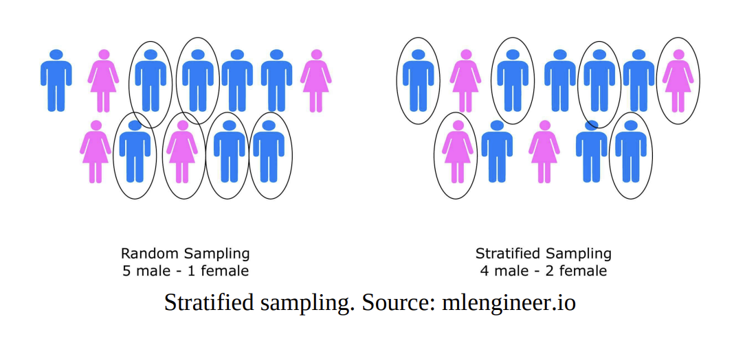
- Use Case: Building a robust test set.
- Problem: You’re building a fraud detection model. Your user base is 70% from the US, 20% from Europe, and 10% from Asia. If you create your test set with pure random sampling, you might get very few examples from Asia, and you won’t have a reliable measure of how well your model performs for that critical segment.
- Solution: You use stratified sampling to build a test set that has the exact 70/20/10 split, guaranteeing a fair evaluation across all geographies.
- The 2024+ Perspective: The principle is more important than ever, especially in the context of Responsible AI and fairness. You must be able to evaluate your model not just on an overall metric, but on its performance across sensitive attributes (age, gender, race, geography). Stratified sampling is the mechanism to create the evaluation datasets that allow you to do this.
- Interview Phrasing: “To ensure our final model performance is robust and fair, we won’t use a simple random split for our test set. Instead, we’ll create it using stratified sampling based on user country. This guarantees that our test set maintains the same geographic distribution as our production traffic, allowing us to confidently measure and report performance for each key region.”
Reservoir Sampling: Sampling from a Stream
- Book’s Core Idea (Timeless): How do you get a uniform random sample of
kitems from a dataset so large you can’t fit it in memory and don’t even know its total size (N) in advance? This is the classic “sampling from a stream” problem. - Intuition & Algorithm (Algorithm R):
- Fill the reservoir: Take the first
kitems from the stream and put them in your reservoir (an array of sizek). - Process the rest: For each subsequent item
i(fromk+1toN):- Generate a random integer
jfrom1toi. - If
jis between1andk, swap thei-th item from the stream with the item at thej-th position in your reservoir. - Otherwise, do nothing (let the
i-th item flow past).
- Generate a random integer
- Fill the reservoir: Take the first
- Why it works: It’s a bit of mathematical magic, but it ensures that at the end of the stream, every item that has ever passed through has had an equal
k/Nprobability of being in the final reservoir. - Diagram:
graph TD
    subgraph "Stream of Unknown Length N"
        I1 --> I2 --> I3 --> I4 --> I5 --> I6 --> I7 --> Etc
    end

    subgraph "Reservoir size k=3"
        R[Reservoir Array]
        R --> RI1
        R --> RI2
        R --> RI3
    end

    subgraph "Step 1: Fill Reservoir"
        I1 --> RI1(Item 1)
        I2 --> RI2(Item 2)
        I3 --> RI3(Item 3)
    end

    subgraph "Step 2: Process Item i=4"
        I4 --> C1[j = random 1 to 4]
        C1 --> Swap[Swap I4 with<br/>item at R j]
        C1 --> Skip1(Do Nothing)
    end

    subgraph "Step 3: Process Item i=5"
        I5 --> C2[j = random 1 to 5]
        C2 --> Swap2[Swap I5 with<br/>item at R j]
        C2 --> Skip2(Do Nothing)
    end

    Etc --> FinalState(Final Reservoir<br/>A random sample of 3 items)
- The 2024+ Perspective: This is a classic algorithm that comes up frequently in coding rounds for data-heavy roles. It’s also used in large-scale data processing systems (like in Spark or Flink) for approximating analytics (e.g., “get me a random sample of 1000 user IDs who performed this action”) without having to do a full, expensive shuffle of the data.
- Interview Phrasing: “If we need to generate a random sample of user sessions from our live Kafka event stream for analysis, we can’t load the whole stream. This is a perfect use case for Reservoir Sampling. We can implement a streaming job that maintains a reservoir of size
k, and for each new event, it probabilistically decides whether to swap it into the reservoir. This gives us a statistically valid, uniform random sample at any point in time without knowing the total size of the stream.”
Topic: Common Deep Learning Model Architectures
1. Wide and Deep Architecture: The Power of Memorization and Generalization
- Book’s Core Idea (Timeless): This is a seminal architecture from Google that elegantly addresses a fundamental tension in recommendation systems:
- Memorization: The system needs to learn and exploit simple, direct rules from the data. For example: “People who searched for ‘iPhone case’ often buy the ‘Apple official silicone case’.” This is about recommending highly related items.
- Generalization: The system needs to explore and discover new, less obvious connections. For example: “People who bought an iPhone case might also be interested in a wireless charger, even if they’ve never shown interest before.” This is about recommending novel items.
- Intuition & Architecture: The Wide & Deep model combines two distinct parts that are joined only at the very end.
- The “Wide” Part (Memorization): This is a simple, linear model (like logistic regression). Its job is to learn the direct, one-to-one feature interactions. It takes in raw features and, most importantly, cross-product features. A cross-product feature is a feature created by combining two others (e.g.,
AND(user_country='USA', item_category='gardening')). This allows the linear model to explicitly memorize the impact of this specific combination. - The “Deep” Part (Generalization): This is a standard feed-forward neural network (MLP). Its job is to take low-dimensional embeddings of the features and discover complex, non-linear, and unseen feature combinations through its hidden layers. It can learn that
user_country='USA'anditem_category='gardening'are correlated withitem_category='bbq_grills'even if very few users have exhibited all three behaviors.
- The “Wide” Part (Memorization): This is a simple, linear model (like logistic regression). Its job is to learn the direct, one-to-one feature interactions. It takes in raw features and, most importantly, cross-product features. A cross-product feature is a feature created by combining two others (e.g.,
graph TD
    subgraph "Input Features"
        Cat_Features[Categorical Features<br/>user_id, item_id, country]
        Num_Features[Numerical Features<br/>price, age]
    end

    subgraph "Wide Part Memorization"
        direction LR
        Cross[Cross-Product<br/>Transform]
        Wide_Model(Simple Linear Model)
        Raw_Features[Raw Features]
        Raw_Features --> Cross
        Cross --> Wide_Model
    end

    subgraph "Deep Part Generalization"
        direction LR
        Embedding(Embedding Layer)
        Deep_Model(Deep Neural Network)
        Embedding --> Deep_Model
    end

    Cat_Features --> Embedding
    Num_Features --> Deep_Model

    subgraph "Output"
        Combine(+)
        Final_Output(Final Prediction<br/>e.g., Sigmoid for p click)
        Combine --> Final_Output
    end

    Wide_Model --> Combine
    Deep_Model --> Combine

    style Cross fill:#fff0b3
    style Embedding fill:#cde4ff
- The 2024+ Perspective: The principle of combining memorization and generalization is more relevant than ever. The Wide & Deep architecture itself is still a very strong baseline. However, the “Deep” side has become more sophisticated (e.g., using attention layers), and the “Wide” side is sometimes replaced or augmented by different explicit feature interaction layers. This leads directly to our next topic…
- Interview Phrasing: “For a search ranking problem with both sparse categorical features and dense numerical features, a Wide & Deep architecture is a great starting point. The ‘wide’ component would allow us to explicitly learn the memorized interactions between key query and item features using cross-product transformations. The ‘deep’ component, operating on learned embeddings, would handle generalization and discover less obvious correlations. This hybrid approach ensures our model is both relevant and capable of novel recommendations.”
2. Two-Tower Architecture: The Scalable Retrieval Champion
- Book’s Core Idea (Timeless): We’ve touched on this before, but let’s formalize it. This architecture is the industry standard for the candidate generation/retrieval stage of any large-scale recommendation or search system (YouTube, Facebook, Pinterest, etc.).
- The Problem it Solves: How do you efficiently find a few hundred “pretty good” candidates from a corpus of billions of items in real-time (under 50ms)? You cannot score every item against the user query.
- Intuition & Architecture: It decouples the query and candidate models.
- Query Tower: Takes in all information about the user and their context (user profile, recent history, time of day) and crunches it down into a single embedding vector (e.g., a 128-dimensional vector).
- Candidate/Item Tower: Takes in all information about an item (title, description, category) and crunches it down into a single embedding vector of the same dimension.
- The Magic (Decoupling): During serving, you can pre-compute the embedding for EVERY item in your corpus and store them in an Approximate Nearest Neighbor (ANN) index like FAISS or a Vector Database. When a user request comes in, you only need to run the lightweight Query Tower to get the user’s embedding. Then, you use that vector to query the ANN index, which very quickly finds the
kitem vectors with the highest dot product similarity.
- Diagram:
graph TD
    subgraph "Query Tower"
        U_Features[User Features<br/>context, history] --> U_L1(Dense Layer)
        U_L1 --> U_L2(Dense Layer)
        U_L2 --> QueryEmbedding[Query Embedding]
    end

    subgraph "Candidate Tower"
        I_Features[Item Features<br/>metadata, text] --> I_L1(Dense Layer)
        I_L1 --> I_L2(Dense Layer)
        I_L2 --> ItemEmbedding[Item Embedding]
    end

    subgraph "Training Objective"
        QueryEmbedding -- Dot Product --> Score
        ItemEmbedding -- Similarity --> Score
        Score --> Loss(Contrastive Loss<br/>e.g., Softmax, Hinge)
    end

    subgraph "Serving / Inference"
        direction LR
        ItemEmbedding --> AllItemEmbeddings[Pre-computed<br/>Item Embeddings]
        AllItemEmbeddings --> ANN_Index[(Vector Database / FAISS<br/>Approximate Nearest Neighbor)]
        QueryEmbedding --> ANN_Index
        ANN_Index --> Top_K_Candidates[Top K Candidates]
    end

    style QueryEmbedding fill:#cde4ff
    style ItemEmbedding fill:#dff0d8
- The 2024+ Perspective: This pattern is now everywhere, not just in classic recommendations. It’s the foundation of Retrieval-Augmented Generation (RAG). The “query tower” is the model that embeds the user’s search query, and the “candidate tower” is the model that embeds the documents in your knowledge base. The principles are identical.
- Interview Phrasing: “To solve the candidate generation problem at scale, I’d design a two-tower retrieval model. We’d have a user/query tower and an item tower, trained jointly with a contrastive loss to map relevant pairs close in the embedding space. The key advantage of this architecture is its serving efficiency. We can pre-compute all item embeddings offline and load them into a vector index. At inference time, we only need to compute the user embedding on-the-fly and query the index to retrieve the top-k candidates in milliseconds.”
3. Deep Cross Network (DCN): Explicit and Bounded Feature Crossing
- Book’s Core Idea (Timeless): DCN is an evolution of the Wide & Deep concept. It asks: “What if we could get the benefits of the ‘wide’ side’s feature crossing, but do it more automatically and efficiently than manually defining cross-products?”
- Intuition & Architecture: DCN replaces the “wide” part with a series of special “cross layers.”
- Each cross layer takes the output from the previous layer
x_iand explicitly calculates its interaction with the original inputx_0. - Equation of a cross layer:
x_{i+1} = x_0 * (w_i^T * x_i) + b_i + x_i - What this means: It’s a very specific mathematical formula designed to create feature crosses of increasing complexity with each layer. Layer 1 creates 2nd-degree interactions, Layer 2 creates 3rd-degree, and so on. The
+ x_iis a residual connection that helps with training stability.
- Each cross layer takes the output from the previous layer
- Diagram: The book’s diagram showing the stacked cross layers is a good representation.
graph TD
    Input --> Embedding

    subgraph "Deep Part (MLP)"
        D1(Dense) --> D2(Dense) --> D_Out
    end

    subgraph "Cross Part (DCN)"
        C1(Cross Layer 1) --> C2(Cross Layer 2) --> C_Out
    end

    Embedding --> D1
    Embedding --> C1

    D_Out --> Combine --> Output
    C_Out --> Combine --> Output

    style C1 fill:#fff0b3
    style C2 fill:#fff0b3
- The 2024+ Perspective: DCN is a very well-respected architecture and a great example to bring up. It shows you know about solutions beyond the original Wide & Deep paper. Its main benefit is creating explicit and bounded-degree feature interactions, which can be more efficient and interpretable than letting a giant MLP learn them implicitly. The latest version, DCNv2, improves the cross-layer to be even more expressive.
- Interview Phrasing: “To improve upon a standard Wide & Deep model, we could explore using a Deep Cross Network (DCN). Instead of manually crafting cross-features for the wide part, DCN uses specialized cross-layers to learn explicit feature interactions of increasing degree automatically. This can be more effective and require less manual feature engineering than the traditional approach.”
4. Multitask Learning: Learning More with Less
- Book’s Core Idea (Timeless): Instead of training separate models to predict different things, can we train a single model to predict all of them at once?
- Intuition & Architecture: The most common pattern is “Shared Bottom” architecture.
- The model has a large, shared set of bottom layers (e.g., the user and item embedding layers and a few shared dense layers). This is where the model learns a general representation of the input.
- The model then splits into multiple small, separate “towers” or “heads,” one for each task. Each tower learns the specific nuances for its own prediction.
- Use Case (YouTube - from the book): A video recommendation model needs to predict multiple outcomes:
- Will the user click on the video? (predict
p(click)) - Will the user like the video? (predict
p(like)) - Will the user subscribe to the channel? (predict
p(subscribe)) - How much watch time will the user generate? (predict
expected_watch_time)
- Will the user click on the video? (predict
- Diagram:
graph TD
    Input[Shared Input Features] --> Shared_Bottom(Shared Layers<br/>e.g., Embeddings, MLP)

    subgraph "Task-Specific Heads"
        Tower_Click(Click Tower)
        Tower_Like(Like Tower)
        Tower_Watch(Watch Time Tower)
        P_Click[Predict p click]
        P_Like[Predict p like]
        P_Time[Predict Watch Time]

        Shared_Bottom --> Tower_Click
        Shared_Bottom --> Tower_Like
        Shared_Bottom --> Tower_Watch
        Tower_Click --> P_Click
        Tower_Like --> P_Like
        Tower_Watch --> P_Time
    end

    subgraph "Total Loss Sum of individual losses"
        L_Click(LogLoss)
        L_Like(LogLoss)
        L_Time(MSE Loss)
        Total_Loss(Combined Loss)

        P_Click --> L_Click
        P_Like --> L_Like
        P_Time --> L_Time
        L_Click --> Total_Loss
        L_Like --> Total_Loss
        L_Time --> Total_Loss
    end
- Why it’s powerful:
- Implicit Regularization: Forcing the model to learn a shared representation that is good for multiple tasks prevents it from overfitting to the idiosyncrasies of any single task. This often leads to better generalization.
- Data Sparsity: It allows tasks with very little data (e.g., “subscribes”) to benefit from the large amount of data available for other tasks (e.g., “clicks”). The shared layers learn from all the data.
- The 2024+ Perspective: This is a core technique in any large-scale system. Modern variants like MMoE (Multi-gate Mixture-of-Experts) improve on the shared-bottom by learning to route information through different “expert” sub-networks based on the input, which is even more powerful. Mentioning MMoE is a strong senior signal.
- Interview Phrasing: “Instead of training separate models to predict clicks and likes, I would build a multi-task learning model. It would have a shared bottom to learn a common user/item representation from all interactions, with separate task-specific heads for predicting
p(click)andp(like). This approach acts as a form of regularization and allows thelikeprediction task, which has sparser data, to benefit from the rich data of theclicktask, likely improving overall model performance.”
Topic: A/B Testing & Experimentation
1. A/B Testing Fundamentals & Budget-Splitting A/B Testing
Book’s Core Idea (Timeless):
- Standard A/B Testing: You split users into two groups. Group A (Control) sees the old model. Group B (Treatment) sees the new model. You compare metrics (CTR, conversions, etc.) between the two groups to declare a winner. This is the gold standard for measuring impact.
- The Problem in Marketplaces (Ads, Search): In a system with a shared, limited resource (like an ad budget or the top spot on a search page), a standard A/B test can be misleading. A “better” model might not be better at all; it might just be more aggressive and “win” the budget from the control group’s model. The overall system revenue might not increase.
- Budget-Splitting A/B Testing: This is LinkedIn’s clever solution to the marketplace problem. Instead of splitting users, you split the budget for each ad campaign. 50% of the budget can only be spent on control group users, and 50% can only be spent on treatment group users. This creates two independent mini-auctions, and you can now fairly compare which model generates more revenue from its allocated budget.
Intuition & Diagram:
graph TD
    subgraph "Standard A/B Test (User Split)"
        U(User Arrives) --> USplit{Is User in Group A or B?}
        USplit -- A --> M_A(Model A)
        USplit -- B --> M_B(Model B)
        M_A & M_B --> Auction{Single Auction<br>Models compete for budget}
        Result_A[Problem: Model B might win<br>just by being more aggressive,<br>not by being better overall.]
    end

    subgraph "Budget-Splitting A/B Test"
        AdCampaign[Ad Campaign<br>Total Budget: $1000] --> BSplit{Split Budget}
        BSplit --> Budget_A(Budget for Control<br>$500)
        BSplit --> Budget_B(Budget for Treatment<br>$500)

        U_A(Control User Arrives) --> M_A2(Model A)
        M_A2 --> Auction_A{Auction A<br>Can only use Budget A}

        U_B(Treatment User Arrives) --> M_B2(Model B)
        M_B2 --> Auction_B{Auction B<br>Can only use Budget B}

        Result_B[Solution: Fair comparison.<br>Does Model B generate more<br>revenue from its $500?]
    end

    style Budget_A fill:#cde4ff
    style Budget_B fill:#dff0d8
The 2024+ Perspective: The core principles are solid. The modern conversation has expanded to include more sophisticated experimental designs.
- Interleaving: For ranking problems, instead of showing a user a full list from Model A or Model B, you can show them a single, blended list containing results from both. You then measure which model’s results the user clicks on more within that blended list. This can be a much faster and more sensitive way to detect ranking improvements.
- Multi-Armed Bandits (Thompson Sampling): For problems where you need to balance exploration (trying new things) vs. exploitation (using the current best option), bandits are key. Instead of a fixed 50/50 traffic split, a bandit algorithm will dynamically allocate more traffic to the better-performing model over time, minimizing regret (lost revenue) during the experiment.
Interview Phrasing: “To test our new ranking model, a standard A/B test would be the first step. However, given this is an ad marketplace, I’d be concerned about budget contention between the control and treatment groups. A more robust approach would be a budget-splitting A/B test to ensure a fair comparison. For faster iteration on ranking quality, we could also consider interleaving, which can detect superior models with less traffic and time. If minimizing revenue loss during the experiment is critical, a multi-armed bandit approach could dynamically allocate traffic to the winning model.”
Topic: Common Deployment Patterns
1. Aggregator / Broker Service for Imbalanced Workload
- Book’s Core Idea (Timeless): You have a complex request that requires scoring a large number of candidates (e.g., 10,000 ads). A single inference server might be too slow to meet the latency requirement (e.g., < 100ms).
- Intuition & Architecture: The Aggregator (or Broker) pattern is a simple “divide and conquer” strategy.
- An Aggregator Service receives the initial request with all 10,000 candidates.
- It splits the list of candidates into smaller chunks (e.g., 10 chunks of 1,000 candidates each).
- It sends these chunks in parallel to multiple Worker Services (the actual model inference servers).
- It waits for all the workers to return their scored chunks.
- It combines the results, does a final sort, and returns the top N candidates.
graph TD
    Client --> Aggregator{Aggregator Service}

    subgraph "Worker Pool (Model Inference)"
        W1(Worker 1)
        W2(Worker 2)
        W3(...)
        WN(Worker N)
    end

    Aggregator -- "Candidates 1-1000" --> W1
    Aggregator -- "Candidates 1001-2000" --> W2
    Aggregator -- "..." --> WN

    W1 -- "Scored chunk" --> Aggregator
    W2 -- "Scored chunk" --> Aggregator
    WN -- "Scored chunk" --> Aggregator

    Aggregator --> FinalResponse(Final Sorted List)
- The 2024+ Perspective: This pattern is fundamental and widely used. It’s essentially a backend-specific load balancer. In a modern Kubernetes environment, the “Worker Pool” would be a set of pods that can be auto-scaled based on the request volume. The key design consideration is handling failures: what if one worker is slow or fails? A robust aggregator needs to have timeouts and potentially a retry mechanism or the ability to return a partial result.
- Interview Phrasing: “A single prediction request involves ranking 10,000 candidates, which would likely exceed our 100ms latency budget if handled by one server. I would implement an aggregator pattern. A front-end service would receive the request, shard the candidate list, and fan out the scoring requests in parallel to a pool of stateless model inference workers. The aggregator would then collect the scored lists, merge them, and return the final ranking. This allows us to scale the number of workers horizontally to meet our latency SLA.”
2. Serving Logic and Multiple Models
- Book’s Core Idea (Timeless): One model doesn’t fit all. You often need business logic to decide which model to use for a given request.
- Example (from the book): An ad serving system might have different models for different user device types.
- If
user_device == 'iOS', route toModel_iOS. - Else, route to
Model_Generic.
- If
- The 2024+ Perspective: This is the foundation of more complex systems.
- Model Ensembles: Instead of just choosing one model, you might route the request to multiple models and then combine their outputs (e.g., by averaging their scores).
- Cascade of Models: For latency-critical funnels, you use a cascade. A very fast, simple model first filters out the 90% worst candidates. The remaining 10% are then passed to a more complex, slower, but more accurate model for the final ranking. This provides the best trade-off between accuracy and speed.
- Diagram (Cascade Example):
graph TD
    Request["Request w/ 100k candidates"] --> M1{"Model 1: Fast and Simple<br/>(e.g., Logistic Regression)"}
    M1 -- "Filters down to 5k candidates" --> M2{"Model 2: Slow and Complex<br/>(e.g., Large Transformer)"}
    M2 -- "Final ranking of top 10" --> Response

    style M1 fill:#cde4ff
    style M2 fill:#dff0d8
- Interview Phrasing: “We could improve performance by implementing a model cascade. A fast, lightweight first-pass model, perhaps a simple logistic regression on basic features, could filter the initial 100,000 candidates down to the top 5,000. Only these promising candidates would then be passed to our larger, more computationally expensive deep learning model for the final re-ranking. This preserves overall accuracy while dramatically reducing the end-to-end latency.”
3. Serving Embeddings
- Book’s Core Idea (Timeless): This section synthesizes many of the previous points, showing how LinkedIn serves its two-tower model. The key distinction is between offline and nearline serving.
- Offline Serving (Batch): For things that don’t change often. For example, a user’s embedding based on their long-term profile. This can be pre-computed in a daily or weekly batch job and stored in a feature store.
- Nearline Serving (Streaming): For things that change quickly. For example, a new job posting is created. This event triggers a streaming process that immediately computes the job’s embedding and makes it available for retrieval.
- The 2024+ Perspective: This is the essence of a modern feature platform.
- Offline (Batch Features): Features computed on a slow cadence (hourly/daily).
user_lifetime_clicks,item_average_rating. - Online (Real-time Features): Features computed on-the-fly at request time, or from a stream processor.
user_clicks_in_last_5_minutes,current_popularity_of_item. - The challenge is joining these features together at inference time with low latency. This is why a high-performance Feature Store is so critical. It’s the system that provides a unified view of both batch and real-time features to the model.
- Offline (Batch Features): Features computed on a slow cadence (hourly/daily).
- Diagram (Feature Store in action):
graph TD
    subgraph "Serving Path"
        Request --> PredictionService{Prediction Service}
        PredictionService --> FeatureStore[(Feature Store)]
        FeatureStore --> Model(ML Model)
        Model --> PredictionService
    end

    subgraph "Batch Pipeline (Offline)"
        DataLake[Data Lake] --> BatchETL{Spark Job}
        BatchETL -- "user_age<br>user_country" --> FeatureStore
    end

    subgraph "Streaming Pipeline (Nearline)"
        EventStream[Kafka Stream] --> StreamProcessor{Flink Job}
        StreamProcessor -- "user_clicks_last_5m" --> FeatureStore
    end

    style FeatureStore fill:#cde4ff,stroke-width:2px,stroke:#333
- Interview Phrasing: “Our model will require both static and dynamic features. Static features, like user profile embeddings, will be pre-computed via a daily batch job and loaded into our online feature store. Dynamic features, like a user’s recent activity in this session, will be computed by a streaming pipeline and also pushed to the feature store. At inference time, our prediction service will query the feature store to assemble the final feature vector from both sources with low latency.”
The Training-Serving Skew Problem (Spotify Case Study)
Book’s Core Idea (Timeless): The case study describes a scenario where a model performs well offline but fails silently in production. The root cause was a subtle difference in how features were processed during training versus during online serving.
The Problem, Deconstructed: Let’s imagine a concrete feature:
user_podcast_listening_history.- Training Pipeline (Offline): A data scientist using a Python script in a Jupyter notebook writes code to process the listening history. Let’s say the logic is: “Take the last 50 podcasts the user listened to, embed their IDs, and average the embeddings.” This pipeline runs on a Spark cluster, reads from the data lake, and produces a training dataset. The model trains on this data and gets great offline metrics.
- Serving System (Online): A different team of backend engineers is responsible for the production service that recommends podcasts. This service is written in Java for low latency. They are given the same instructions: “Take the last 50 podcasts, embed, and average.” They re-implement this feature transformation logic in Java.
- The “Simple Mistake”: The Python
split()function might handle a missing history differently than the Javasplit()function. Or maybe the Java service, in a rare edge case, only has access to the last 49 podcasts due to a cache refresh issue. Or maybe the Python script defaults to zero-padding while the Java service doesn’t. - The Result: The live production model is consistently receiving feature vectors that are calculated slightly differently than the vectors it was trained on. The model is making predictions on data that it doesn’t quite understand, leading to poor (but not catastrophically bad) recommendations. Because the failure isn’t a crash, it goes undetected for months, silently hurting user experience. This is training-serving skew.
Diagram of the Failure Mode:
graph TD
    subgraph "Training World (Python/Spark)"
        A[Data Lake] --> B{Feature Transform v1<br><span style='color: blue;'>Python Logic</span>}
        B --> C[Training Data]
        C --> D(Model Training)
        D --> E[(Saved Model)]
    end

    subgraph "Serving World (Java/Real-time)"
        F[Live User Request] --> G{Feature Transform v2<br><span style='color: red;'>Java Logic</span>}
        G --> H[Inference Feature Vector]
        E --> I{Model Inference}
        H --> I
        I --> J(Recommendation)
    end

    subgraph "The Problem"
        Skew("Training-Serving Skew<br>Transform v1 ≠ Transform v2")
    end

    style B fill:#cde4ff
    style G fill:#f5c6cb
Solutions to Training-Serving Skew
The book highlights Spotify’s solution, which is excellent. Let’s break down the modern best practices for solving this, which have become industry standard.
Solution 1: The Feature Store (The “Source of Truth” Approach)
This is the most robust, architectural solution and the one we discussed previously.
- How it solves the problem: You create a single, canonical feature engineering pipeline. This pipeline computes features and writes them to both an offline store (for training) and an online store (for serving).
- The model training job reads directly from the offline store.
- The model serving service reads directly from the online store.
- There is no re-implementation of feature logic. The logic is defined once. This completely eliminates the possibility of implementation drift between training and serving.
- Diagram of the Solution:
graph TD
    subgraph "Canonical Feature Pipeline (Defined ONCE)"
        A["Raw Data Source"] --> B{"Feature Transform Logic<br/>(Spark/Flink)"}
        B -- "Writes to" --> C[("Online Feature Store<br/>Redis, DynamoDB")]
        B -- "Writes to" --> D[("Offline Feature Store<br/>S3/Iceberg")]
    end

    subgraph "Training World"
        D -- "Reads clean features" --> Model_Training("Model Training")
    end

    subgraph "Serving World"
        C -- "Reads clean features" --> Model_Serving("Model Serving")
    end

    style B fill:#dff0d8
Solution 2: The Shared Transformation Library Approach
This is a lighter-weight solution if a full feature store is overkill.
- How it solves the problem: You encapsulate all your feature transformation logic into a dedicated library that can be used by both the training and serving environments.
- Example (TensorFlow Transform - TFX): You define your feature preprocessing steps (normalization, vocabulary creation, etc.) using TFX. TFX analyzes your entire training dataset to compute the necessary statistics (e.g., the mean and variance for normalization). It then exports two things:
- The transformed data for training.
- A
transform_fngraph that contains all the logic and the computed statistics.
- Your serving system simply loads this
transform_fngraph and applies it to the raw incoming data. There’s no re-implementation. The exact same means, standard deviations, and vocabularies are used in both worlds.
Solution 3: The Logging and Monitoring Approach
This is not a preventative solution, but a detection and alerting solution. You must do this even if you have one of the above.
How it works:
- Log Predictions and Features: Your online serving system logs every feature vector it uses to make a prediction, along with the prediction itself, to a central data lake.
- Statistical Monitoring: You set up a separate pipeline that runs periodically (e.g., hourly) and compares the statistical distribution of the features from the production logs against the distribution of the features from your training data.
- Tools: Libraries like TensorFlow Data Validation (TFDV) or open-source tools like WhyLogs/whylogs are purpose-built for this. They can automatically generate schemas and detect anomalies.
- Alerting: If the monitoring pipeline detects a feature drift or concept drift (e.g., the mean of
user_agein production suddenly shifts significantly from the training data, or the distribution of predicted scores changes), it triggers an alert for the on-call engineer.
The book’s mention of the Chebyshev distance metric is a great specific detail to include here.
Interview Phrasing: “Training-serving skew is one of the most insidious failure modes in production ML. My primary strategy to prevent it would be to use a Feature Store, which provides a single source of truth for both training and serving features. This architecturally eliminates the need to re-implement feature logic. As a crucial second layer of defense, I would implement a monitoring and alerting pipeline. The production service would log all its input feature vectors, and a separate job using a tool like TFDV would compare the statistical distributions of these live features against our training set’s features. If any significant drift is detected, it would trigger an on-call alert, allowing us to catch issues like the one Spotify faced in hours, not months.”